Tuesday, April 24, 2012

JPEG VS JPEG 2000


What is JPEG?
  • Joint Photographic Experts Group (pronounced JAY-pehg).
  • An ISO/ITU standard for compressing still images
  • File extensions are .JPEG, .JFIF, .JPG, OR .JPE
  • Uses Discrete Cosine Transform (DCT) algorithm.
  • Lossy coding of continuous tone still images.
  • Very popular due to its variable compression range.
  • Best for compressing photographic images (compared to GIFs).
  • Mostly used for storing and transmitting photographs on the World Wide Web

Advantages of JPEG:
    • low complexity
    • memory efficient
    • reasonable coding efficiency
    • currently applicable for most applications
    • can be saved on a sliding resolution scale based on the quality desired

Disadvantages of JPEG:
    • not great for text - the text appears fuzzy, especially at low resolutions
    • lossy - some data or quality is lost when the image is compressed


What is JPEG 2000?
  • New format of JPEG formalised in December 2000.
  • File extensions : .jp2, .jpx, .jpf, .mj2
  • A revolutionary image compression standard based on wavelet technology and is replacing the old JPEG format.
  • Uses Discrete Wavelet Transform (DWT)
  • Scalable coding of continuous tone still images (from lossy to lossless).
  • Provides both lossless and lossy compression in a single compression architecture

Advantages of JPEG 2000:
    • Better image quality at the same file size
    • 25%–35% smaller file sizes at comparable image quality.
    • Good image quality even at very high compression ratios, over 80:1.
    • Lossless compression mode (identical to original image).

Disadvantages of JPEG 2000:
    • appropriate program or plugin is needed to view
    • more demanding in memory
    • consume higher computation time


JPEG VS JPEG 2000


JPEG
JPEG 2000
  • Created for natural imagery
  • Created for computer generated imagery
  • Discrete Cosine Transform (DCT) algorithm
  • Discrete Wavelet Transform (DWT) algorithm
  • File Extensions:
    • .jpeg
    • .jfif
    • .jpg
    • .jpe
  • File extention :
    • .jp2
    • .jpx
    • .jpf
    • .mj2
  • Currently applicable to most of  applications
  • Currently NOT widely used
Main Differences between JPEG and JPEG 2000


Tuesday, April 3, 2012

[Lab03] Intensity Transformation and Spatial Filter Part 2


Spatial Filtering

In the previous post, we have learned about intensity transformation. This post will be focus on another principal category for image processing – Spatial Filtering. Filter (or known as Mask) refers to “accepting” or “rejecting” a certain frequency components. These accepting or rejecting is known as smoothing or sharping.

Spatial Filtering is also known as neighbourhood processing. This is because we define a center point and apply a filter to only the neighbours of the center point. The result of the operation is one value which will become the new value of the center point in the modified image. In short, the process of spatial filtering simply consists of moving the mask from point to point in an image to derive the new value of the pixel.

Basic idea :
  • Size of neighbourhood = size of mask.
  • Mask slides from left to right, top to bottom.
  • Same operation is performed on every pixel. 
  • Neighbourhood exceeds image boundary = zero padding or replication of border pixel.  


Using myfilter.m

Let us try out spatial filtering using MATLAB. First, we need to create a MATLAB file (M-file) and save it as myfilter.m. Copy and paste the code below in the file. The MATLAB code below was written by Nova Scheidt:

% MYFILTER performs spatial correlation
% I = MYFILTER(f,w) produces an image that has undergone correlation
% f is the original image
% w is the filter (assumed to be 3x3)
% the original image is padded with 0's

function img = myfilter(f,w)
% check that the filter,w is 3x3
[m,n] = size(w);

if m~=3 || n~=3
   error ('Filter must be 3x3') 
end

% get size of the original image, f
[x,y] = size(f);

% create padded f (namely g)  
% filled with zeros
g = zeros (x+2, y+2);

% store f withing g
for i = 1:x
    for j = 1:y
        g(i+1, j+1) = f(i,j);  
    end 
end

% traverse the array and apply the filter
for i = 1:x
    for j = 1:y
        img(i,j) = g(i,j)*w(1,1) + g(i+1,j)*w(2,1) + g(i+2,j)*w(3,1)...
           + g(i,j+1)*w(1,2) + g(i+1,j+1)*w(2,2) + g(i+2,j+1)*w(3,2)...
           + g(i,j+2)*w(1,3) + g(i+1,j+2)*w(2,3) + g(i+2,j+2)*w(3,3);  
    end 
end

% convert to uint -- expected range is [0,1] when the image is displayed
img = uint8(img);
end

To apply this filter, we need to create an average filter (for this lab, we are using 3x3 matrix). The following code are used to do the filtering. By using the imtool, we can zoom out the picture for clearer result. The picture below have been zoomed 3000%.

% create average filter
>> w = [1/9, 1/9, 1/9; 1/9, 1/9, 1/9,; 1/9, 1/9, 1/9];

% applying the filter to an image
>> original_img = imread('stock_cut.jpg');
>> results = myfilter(original_img, w);
>> imtool(results)  


Using imfilter


Instead of using the M-file, we can use a function that comes as part of the Image Processing Toolkit. To use it, we need to call imfilter as below:

% create average filter
>> w = [1/9, 1/9, 1/9; 1/9, 1/9, 1/9,; 1/9, 1/9, 1/9];

% applying the filter to an image
>> original_img = imread('stock_cut.jpg');
>> results2 = imfilter(original_img, w);
>> imtool(results2)  


Using imfilter – with boundary options

The imfilter comes with a various boundary options. The following table shows the summary of additional options available (sources from Digital Image Processing, Using MATLAB, by Rafael C. Gonzalez, Richard E.Woods,and Steven L.Eddins).  


Since we are considering neighbourhood pixel, there are some cases where we there are no upper or lower neighbours or neighbours to the left or right. These are usually occurs when the mask covers the neighbourhood that exceeds the image boundary. For example, based on the image above, there are no upper neighbours or neighbours to the left. In order to solve this, we have two solutions- Zero padding and replicating.

Let us try the imfilter with different boundary options. The code below includes zero padding, replication, symmetric and circular. We are using 5 x 5 filter for clearer result.

% create a 5x5 average filter
>> h = fspecial('average', 5);

% zero-padding
>> results1 = imfilter(cat,h);

% replication
>> results2 = imfilter(cat,h,'replicate');

% symmetric
>> results3 = imfilter(cat,h,'symmetric');

% circular
>> results4 = imfilter(cat,h,'circular');


>> figure, imshow(cat)
>> title('Original');
>> figure, imshow(results1)
>> title('Zero-Padded');
>> figure, imshow(results2)
>> title('Replicate');
>> figure, imshow(results3) 
>> title('Symmetric');
>> figure, imshow(results4)
>> title('Circular');  


Using imfilter – with filtering mode

With imfilter, we can choose one of the two filtering modes: correlation or convolution. Correlation is the default. Convolution rotates the filter by 180 degree before performing multiplication. The diagram below demonstrates correlation versus convolution operation.  


Let us try out the filtering mode and see what happen to the images after we applied the filtering mode. Below is the sample of MATLAB code that we can try:

>> h = [1 2 3; 4 5 6; 7 8 9];
>> h = h/45; 

% correlation mode
% or we can use imfilter(cat,h,'conv');
>> result_corr = imfilter(cat,h);

% convolution mode
>> result_conv = imfilter(cat,h,'conv');
>> figure, imshow(result_conv)
>> title('Convolution')
>> figure, imshow(result_corr)
>> title('Correlation')  


Using imfilter – size option

There are two size options – full or same. ‘full’ option will be as large as the padded image, while ‘same’, which is the default, will be the same size as the input image. Below are the codes that demonstrate the application of size option for imfilter. Notice that ths ‘same’ is 16x16 whereas ‘full’ 18x18.

% create a 3x3 average filter
>> h = [1/9, 1/9, 1/9; 1/9, 1/9, 1/9,; 1/9, 1/9, 1/9];

% same option
>> stock_cut_same = imfilter(original_img,h);

% full option
>> stock_cut_full = imfilter(original_img,h, 'full');


>> figure, imtool(stock_cut_same) >> figure, imtool(stock_cut_full)  


[Lab03] Intensity Transformation and Spatial Filter Part 1

Untitled Document


Intensity Transformation Functions


Intensity transformation involves contrast manipulation and thresholding. An application of intensity transformation is to increase the contrast between certain intensity values so that we can the information that we seek is more visible and clear.

Making changes in the intensity is done through Intensity Transformation Functions. The four main intensity transformation functions are:
  • Photographic Negative
  • Gamma Transformation
  • Logarithmic Transformation
  • Contrast-stretching Transformation


Photographic negative


To use Photographic Negative, use MATLAB function called imcomplement . With this transformation, the true black become true white and vice versa. It is suitable when the black areas are dominant in size. Below are the codes that implements photographic negative and example of photographic negative images.

>> I = imread('cat.jpg');
>> imshow(I)
>> J=imcomplement(I);
>> figure,imshow(J)


The following plots the photographic negative.


Gamma Transformation 


To use Gamma Transformation, use MATLAB function called imadjust. The syntax of this function is:

J = imadjust(f,[low_in high_in],[low_out high_out], gamma)
where :
f = input image
[low_in high_in],[low_out high_out] = for clipping
gamma = controls the curve


Values for low_in, high_in, low_out, and high_out must be between 0 and 1. Values below low_in are clipped to low_out and values above high_in are clipped to high_out. For the example below, we will use empty matrix ([]) to specify the default of [0 1].

gamma specifies the shape of the curve describing the relationship between the values in J and f. If gamma is less than 1, the mapping is weighted toward higher (brighter) output values. If gamma is greater than 1, the mapping is weighted toward lower (darker) output values. By default, gamma is set to 1 (linear mapping).

Below are the codes that implements gamma transformation and example of gamma transformation images.

>> I = imread('cat.jpg');
>> J1 = imadjust(I,[],[],3);
>> J2 = imadjust(I,[],[],1);
>> J3 = imadjust(I,[],[],0.4);
>> imshow(J1);
>> figure, imshow(J2);
>> figure, imshow(J3);


The following plots the gamma transformations with varying gamma.


Logarithmic Transformation


To use Logarithmic Transformation, use the function c*log(1+f).This transformation enhances the details (or contrast) in the darker region of an image (with lower intensity values) by expensing detail in brighter regions. In other words, it expands the values of dark pixel in an image while compressing the higher level values. The syntax of this function is :

g = c*log(1+double(f))

The higher the c, the brighter the image will appear. Any values (produced from logarithmic transformation) greater than one, are displayed as full intensity, equivalent to the value of 1. Below are the codes that implements logarithmic transformation and example of logarithmic transformation images.

>> imshow(I)
>> I2 = im2double(I);
>> J4 = 1 * log(1 + I2);
>> J5 = 2 * log(1 + I2);
>> J6 = 5 * log(1 + I2);
>> figure, imshow(J4)
>> figure, imshow(J5)
>> figure, imshow(J6)


The following plots the logarithmic transformations with varying C.


Contrast-Stretching Transformation


Contrast-Stretching Transformation (also called Piecewise-Linear Transformation) stretches gray-level ranges where we desire more information. This transformation increases the contrast between the darks and the lights. In simple words, the dark becomes darker and the light becomes brighter. To use this transformation, we use the function as below:

g = (1./(1+(m./(double(f)+eps)).^ E)


where:
E = slope function
m = mid-line of switching from dark value to light value
eps = MATLAB constant; distance between 1.0 and the next largest number in double-precision floating point [2^(-52)]


            Below are the codes that use contrast-stretching transformation. The mean of the image intensities as m value and varies the value of E. The higher the value of E, the function becomes more like a thresholding function, which results the image is more black and white than grayscale.

>> I=imread('cat.jpg');
>> I2=im2double(I);
>> m=mean2(I2)
>> contrast1 = 1./(1 + (m ./(I2 + eps )).^4);
>> contrast2 = 1./(1 + (m ./(I2 + eps )).^5);
>> contrast3 = 1./(1 + (m ./(I2 + eps )).^10);
>> contrast4 = 1./(1 + (m ./(I2 + eps )).^-5);
>> contrast5 = 1./(1 + (m ./(I2 + eps )).^-1);
>> figure, imshow(I2)
>> figure, imshow(contrast1)
>> figure, imshow(contrast2)
>> figure, imshow(contrast3)
>> figure, imshow(contrast4)
>> figure, imshow(contrast5)


The following plots the gamma transformations with varying E.


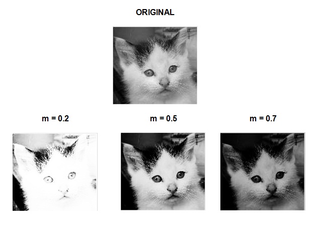
Another contrast-stretching transformation being applied by setting the value of E and to 4 and varies the value of m. The higher the value of m, the darker the image and fewer details are showed.

>> I=imread('cat.jpg');
>> I2=im2double(I);
>> contrast6 = 1./(1 + (0.2 ./(I2 + eps )).^4);
>> contrast7 = 1./(1 + (0.5 ./(I2 + eps )).^4);
>> contrast8 = 1./(1 + (0.7 ./(I2 + eps )).^4);
>> figure, imshow(I2)
>> figure, imshow(contrast6)
>> figure, imshow(contrast7)
>> figure, imshow(contrast8)


The following plots the contrast-stretching transformations with varying m.

Tuesday, March 27, 2012

[Lab02] Image Acquisition and Basic Operation

Image Acquisition

Take any picture of anything you like by using a digital camera and transfer the picture from your camera to your computer. The image should be able to view it by standard image viewing software such as Windows Picture and Fax Viewer).


Read the image into MATLAB

>> x = imread (‘obama.png’);


Display the Information

>> whos x
Name      Size          Bytes     Class    Attributes
     x         278x200x3     166800    uint8             

The class should be “unit8” and the 3rd dimension of size of x should be 3 which denote it is a colour image which correspond the three components which are Red, Green and Blue channels.


Red       x(:,:,1)
Green     x(:,:,2)
Blue      x(:,:,1)

The first colon denotes all rows, the second colon all columns, and the third index denotes the color (1 for red, 2 for green and 3 for blue).


Display the image    

>> imshow(x)


Convert Color Image to Grayscale


>>x_g = rgb2gray(x);
>>figure, imshow(x_g)

rgb2gray command converts the truecolor image RGB to the grayscale intensity image. rgb2gray converts RGB images to grayscale by eliminating the hue and saturation information while retaining the luminance.


Display R, G or B Channel of the Image

There are many ways to display an image in certain channel (red, green or blue channel). You can try either:

  • clear or set the other channels to 0
  • using colormap


For the first option, we need to assign a different variable for the image so that we do not overwrite the original image. As for the example below, we assigned image x to three different variables (x_green, x_red and x_blue for green, red and blue channel respectively).


Red
>>x_red = x;
>>x_red(:,:,2) = 0;
>>x_red(:,:,3) = 0;
Green
>>x_green = x;
>>x_green(:,:,1) = 0;
>>x_green(:,:,3) = 0;
Blue
>>x_blue = x;
>>x_blue(:,:,1) = 0;
>>x_blue(:,:,2) = 0;


Take note that (:,:,1) represent red channel, (:,:,2) represents green channel and (:,:,3) represents blue channel . So, if we want to display the red channel, we must set the green and blue channel to 0 and vice versa.

For the second option, we need to extract each of these layers by using their respective indices (Red = 1, Green = 2, Blue = 3).

>>img_r = I(:,:,1);
>>image(img_r), colorbar;


The image above shows red channel of image x. By default, the colorbar has a scale of 0 to 64. It is difficult to use this rainbow-colored scale. The color intensity for full-color images ranges is from 0 to 255. Thus, we need to modify the scale by using colormap. This can be done as below.

Red
>>R = x(:,:,1);
>>figure;
>>image(R),colormap([[0:1/255:1]',zeros(256,1),zeros(256,1)]), colorbar;

Green
>>G = x(:,:,2);
>>figure;
>>image(G),colormap([zeros(256,1),[0:1/255:1]',zeros(256,1)]), colorbar;

Blue
>>B = x(:,:,3);
>>figure;
>>image(B),colormap([zeros(256,1),zeros(256,1),[0:1/255:1]']),colorbar;


Transpose an Image

To transpose the image, use imshow command followed by the variable name with apostrophe ( ).

>>imshow(x_g');


Crop an Image

To crop an image, use imcrop command followed by the variable name and the size of the crop rectangle, rect. rect is a four-element position vector [xmin ymin width height] that specifies the size and position of the crop rectangle.

>> cropImg = imcrop(x_g,[1 1 100 100]);
>> figure, imshow (cropImg);


Flip an Image

To flip an image, use flipdim command followed by the variable and number of 1 (vertically) or 2 (horizontally)

>>upsidedown=flipdim(x_g,1);
>>figure,imshow(upsidedown);


>>left2right=flipdim(x_g,2);
>>figure,imshow(left2right);

.

[Lab01] Image Processing Toolbox


Reminder: This blog ONLY covers basics that are related to Image Processing. For further information, you are recommended to read the MATLAB Getting Started documentation. Make sure that your MATLAB has been installed Image Processing Toolbox. For information about installing the toolbox, see the MATLAB Installation Guide.


Read an Image
To read an image, use the imread command followed by the name of the image with its extension as an argument. For example below, we are assigning an image named Porsche.tiff to a variable, I:


>>I = imread('Porsche.tiff');


Display an Image
To display the image that we have read, use the imshow command followed by the variable as an argument. A popup window will appeared with the image stored in the variable. Example below will display the image stored in variable I.

>>imshow(I);


Check the Image in Memory
To check how the files are stored in memory, use whos command. As for this case, only I is only stored in the memory, so MATLAB responds with the result of I. These files also can be easily seen in the workspace on the right panel of your MATLAB (this might be different with you MATLAB interface. If you do not have workspace panel, go to Desktop >> Workspace)


>>whos

Name       Size         Bytes     Class    Attributes

I         342x546       186732    uint8             


Perform Histogram Equalization
To see the distribution of intensities of the image stored in I, use imhist command followed by the variable I as the argument. For example below, we use figure command to open new figure window and display the histogram.


>>figure, imhist(I)


To spread the intensity values over the full range, use histeq command followed by the variable as the argument. In result, the image will be more contrast. This command is useful if the histogram produced by imhist command gives narrow intensity range.


>>I2 = histeq(I)
>>figure, imshow(I2)


Write the Image
To write the image I2, the image I that we have adjusted, in simple words, we would like to save the image to the disk, use imwrite command followed by the argument consists of the variable and the name and the extension that you want the image saved as. For example below, we would like to save the I2 image as Porsche2.png.

>>imwrite (I2, Porsche2.png’)


Check the Contents of the File
To check the contents of the file, use imfinfo command followed by the name of the file with its extension as the argument. The example below checks the content the newly written file.

>>imfinfo(‘Porsche2.png’)
ans =

                  Filename: [1x100 char]
               FileModDate: '13-Mar-2012 16:50:08'
                  FileSize: 71980
                    Format: 'png'
             FormatVersion: []
                     Width: 546
                    Height: 342
                  BitDepth: 8
                 ColorType: 'grayscale'
           FormatSignature: [137 80 78 71 13 10 26 10]
                  Colormap: []
                 Histogram: []
             InterlaceType: 'none'
              Transparency: 'none'
    SimpleTransparencyData: []
           BackgroundColor: []
           RenderingIntent: []
            Chromaticities: []
                     Gamma: []
               XResolution: []
               YResolution: []
            ResolutionUnit: []
                   XOffset: []
                   YOffset: []
                OffsetUnit: []
           SignificantBits: []
              ImageModTime: '13 Mar 2012 08:50:07 +0000'
                     Title: []
                    Author: []
               Description: []
                 Copyright: []
              CreationTime: []
                  Software: []
                Disclaimer: []
                   Warning: []
                    Source: []
                   Comment: []
                 OtherText: []