[Lab03] Intensity Transformation and Spatial Filter Part 2

Spatial Filtering

In the previous post, we have learned about intensity transformation. This post will be focus on another principal category for image processing – Spatial Filtering. Filter (or known as Mask) refers to “accepting” or “rejecting” a certain frequency components. These accepting or rejecting is known as smoothing or sharping.

Spatial Filtering is also known as neighbourhood processing. This is because we define a center point and apply a filter to only the neighbours of the center point. The result of the operation is one value which will become the new value of the center point in the modified image. In short, the process of spatial filtering simply consists of moving the mask from point to point in an image to derive the new value of the pixel.

Basic idea :

• Size of neighbourhood = size of mask.
• Mask slides from left to right, top to bottom.
• Same operation is performed on every pixel. 
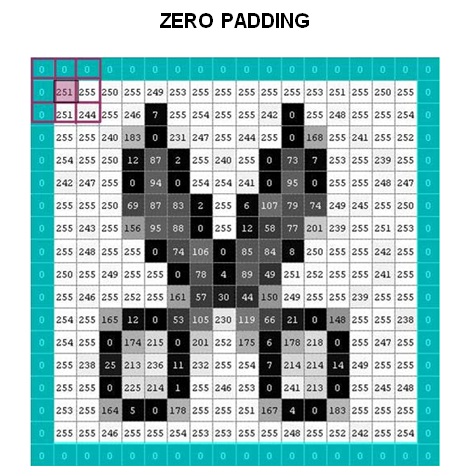
• Neighbourhood exceeds image boundary = zero padding or replication of border pixel.  

Using myfilter.m

Let us try out spatial filtering using MATLAB. First, we need to create a MATLAB file (M-file) and save it as myfilter.m. Copy and paste the code below in the file. The MATLAB code below was written by Nova Scheidt:

% MYFILTER performs spatial correlation
% I = MYFILTER(f,w) produces an image that has undergone correlation
% f is the original image
% w is the filter (assumed to be 3x3)
% the original image is padded with 0's

function img = myfilter(f,w)
% check that the filter,w is 3x3
[m,n] = size(w);

if m~=3 || n~=3
   error ('Filter must be 3x3') 
end

% get size of the original image, f
[x,y] = size(f);

% create padded f (namely g)  
% filled with zeros
g = zeros (x+2, y+2);

% store f withing g
for i = 1:x
    for j = 1:y
        g(i+1, j+1) = f(i,j);  
    end 
end

% traverse the array and apply the filter
for i = 1:x
    for j = 1:y

        img(i,j) = g(i,j)*w(1,1) + g(i+1,j)*w(2,1) + g(i+2,j)*w(3,1)...

           + g(i,j+1)*w(1,2) + g(i+1,j+1)*w(2,2) + g(i+2,j+1)*w(3,2)...

           + g(i,j+2)*w(1,3) + g(i+1,j+2)*w(2,3) + g(i+2,j+2)*w(3,3);  

    end 
end

% convert to uint -- expected range is [0,1] when the image is displayed
img = uint8(img);
end

To apply this filter, we need to create an average filter (for this lab, we are using 3x3 matrix). The following code are used to do the filtering. By using the imtool, we can zoom out the picture for clearer result. The picture below have been zoomed 3000%.

% create average filter
>> w = [1/9, 1/9, 1/9; 1/9, 1/9, 1/9,; 1/9, 1/9, 1/9];

% applying the filter to an image
>> original_img = imread('stock_cut.jpg');
>> results = myfilter(original_img, w);
>> imtool(results)  

Using imfilter

Instead of using the M-file, we can use a function that comes as part of the Image Processing Toolkit. To use it, we need to call imfilter as below:

% create average filter
>> w = [1/9, 1/9, 1/9; 1/9, 1/9, 1/9,; 1/9, 1/9, 1/9];

% applying the filter to an image
>> original_img = imread('stock_cut.jpg');
>> results2 = imfilter(original_img, w);
>> imtool(results2)  

Using imfilter – with boundary options

The imfilter comes with a various boundary options. The following table shows the summary of additional options available (sources from Digital Image Processing, Using MATLAB, by Rafael C. Gonzalez, Richard E.Woods,and Steven L.Eddins).  

  

Since we are considering neighbourhood pixel, there are some cases where we there are no upper or lower neighbours or neighbours to the left or right. These are usually occurs when the mask covers the neighbourhood that exceeds the image boundary. For example, based on the image above, there are no upper neighbours or neighbours to the left. In order to solve this, we have two solutions- Zero padding and replicating.

Let us try the imfilter with different boundary options. The code below includes zero padding, replication, symmetric and circular. We are using 5 x 5 filter for clearer result.

% create a 5x5 average filter
>> h = fspecial('average', 5);

% zero-padding
>> results1 = imfilter(cat,h);

% replication
>> results2 = imfilter(cat,h,'replicate');

% symmetric
>> results3 = imfilter(cat,h,'symmetric');

% circular
>> results4 = imfilter(cat,h,'circular');


>> figure, imshow(cat)
>> title('Original');
>> figure, imshow(results1)
>> title('Zero-Padded');
>> figure, imshow(results2)
>> title('Replicate');
>> figure, imshow(results3) 
>> title('Symmetric');
>> figure, imshow(results4)
>> title('Circular');  

Using imfilter – with filtering mode

With imfilter, we can choose one of the two filtering modes: correlation or convolution. Correlation is the default. Convolution rotates the filter by 180 degree before performing multiplication. The diagram below demonstrates correlation versus convolution operation.  

Let us try out the filtering mode and see what happen to the images after we applied the filtering mode. Below is the sample of MATLAB code that we can try:

>> h = [1 2 3; 4 5 6; 7 8 9];
>> h = h/45; 

% correlation mode
% or we can use imfilter(cat,h,'conv');
>> result_corr = imfilter(cat,h);

% convolution mode
>> result_conv = imfilter(cat,h,'conv');
>> figure, imshow(result_conv)
>> title('Convolution')
>> figure, imshow(result_corr)
>> title('Correlation')  

Using imfilter – size option

There are two size options – full or same. ‘full’ option will be as large as the padded image, while ‘same’, which is the default, will be the same size as the input image. Below are the codes that demonstrate the application of size option for imfilter. Notice that ths ‘same’ is 16x16 whereas ‘full’ 18x18.

% create a 3x3 average filter
>> h = [1/9, 1/9, 1/9; 1/9, 1/9, 1/9,; 1/9, 1/9, 1/9];

% same option
>> stock_cut_same = imfilter(original_img,h);

% full option
>> stock_cut_full = imfilter(original_img,h, 'full');


>> figure, imtool(stock_cut_same) >> figure, imtool(stock_cut_full)